Table of Contents
Introductory Lab: Franck-Hertz Critical Potentials
In the early twentieth century, physicists found themselves surrounded by many physical observations that could not be explained by Classical Mechanics – including the optical spectra emitted by atoms and molecules, blackbody radiation, and the photoelectric effect. It was a time in which the models proposed by theorists (like Einstein, Bohr, and Plank) influenced the tests carried out by experimentalists (like Franck and Hertz)… and vice versa.
Only through this back and forth (observation, modeling, testing, revision, etc.) did Quantum Mechanics emerge as the explanation of the universe that we rely on today.
The Franck-Hertz Critical Potential experiment is the first direct measurement of electron transition energies in atoms. Though there had been significant previous work measuring the discrete wavelengths of light emitted by hot gases and models for the quantization of light into photons, it was not until these results (and, in fact, not until the reinterpretation of these results, since Franck and Hertz initially drew the wrong conclusions) that physicists had clear evidence of the connection between wavelength, frequency, and energy in light: $E = hf = hc/\lambda$.
Learning goals
By the end of this experiment, students are expected to be able to do the following:
Technical:
- Perform basic wiring, and use measurement tools like a multimeter and oscilloscope
- Use advanced scope techniques (like high frequency reject triggering, averaging, using cursors, and saving traces)
- Keep a lab notebook (with a focus on keeping track of multiple data sets and saved files; noting settings, procedure and calibration information; and making quick back-of-the-envelope calculations in-lab).
Data Collection:
- Calibrate from measured quantities (e.g. $V_{scope}$) to desired quantities (e.g. electron kinetic energy).
- Make choices about apparatus settings to obtain “optimal” data (e.g. setting voltage ramp limits, tuning filament current, and adjusting scope triggering/averaging)
- Estimate uncertainties from scope data (including considerations of skew due to features on a sloped background)
Analysis:
- Import and re-plot data files (with annotations)
- Fit linear data
- Use a calibration formula to convert quantities
- Propagate uncertainties to calculated quantities
- Compare values to literature
Topics explored
Students will gain exposure to and practice with the following topics:
Experimental topics covered:
- Measurable (and correctable) systematic biases
- Smearing of features due to resolution effects
- Techniques to enhance signal-to-noise
Physics topics covered:
- Atomic Physics: energy level structure of helium, parahelium vs. orthohelium, inelastic electron collisions, electronic excitation, selection rules, ionization, and wavelength-energy conversion
- Electricity and Magnetism: acceleration of electrons and charged He+ ions
- Electronics: circuit with multiple voltage sources, floating power supplies, voltage dividers, 60 Hz noise, and important grounding considerations
- Experiment Design: use of an oscilloscope to measure short time signals, grounding and noise considerations, interpretation of signals with multiple contributing physics effects, apparatus considerations (e.g. accelerating voltage choices, helium gas density in the tube, current saturation, signal amplification)
- Physics History: history of the development of atomic physics and quantum mechanics
Before you come to lab...
To prepare for each lab this year, you will be asked to read over some preliminary information (theory, background, motivation, etc.) and answer some questions. This prelab assignment will be included on all experiments, but the questions and readings will be tailored to each experiment to make sure you are prepared to start working as soon as you get to lab.
Before coming to lab, read the information below and complete the exercises that follow in a separate document. You will not be graded on whether you get every question correct, but you will be evaluated on whether you made a satisfactory effort to complete these questions before lab.
The prelab assignment is due before lab begins and should be submitted to Canvas. There are no exceptions. (For example, if your lab begins at 1:30 pm and you submit at 1:31 pm, you will receive zero credit.)
Background
In 1900, Max Planck attempted to establish a firm theoretical foundation for understanding the blackbody radiation spectrum. In order to do so, he reluctantly introduced the idea that electrons in the walls of a black body cavity emitted energy (in the form of light) that was quantized in multiples of some elementary unit. Despite this quantization of energy, Planck still believed that the light traveled outward in a continuous wave.
In 1905, in his study of the photoelectric effect, Albert Einstein found that more generally any traveling light wave (not just that emitted by blackbody radiation) is composed of these discrete chunks. Together, their work established that photons of light carry energy $E=hf = hc/\lambda$, where $f$ is the frequency of the light, $\lambda$ is the wavelength, $c$ is the speed of light, and $h$ is now called Planck's constant.
In 1913, Niels Bohr introduced his model of the hydrogen atom, which included the concept of discrete (quantized) energy states. In Bohr’s model, transitions from one energy state to another would help explain the discrete lines observed in the emission spectra of the elements. However, when measuring spectral lines with a diffraction grating spectrometer (assuming a wave nature of light), one is measuring wavelengths, not energies. Therefore, the relationship between energy and wavelength (or frequency) still remained only theoretical, not tested by experiment.
In 1914, James Franck and Gustav Hertz demonstrated that atoms in a gas may absorb energy due to collisions with electrons and that this transfer of energy always occurs in discrete, measurable amounts. At the time of their work, Franck and Hertz were apparently unaware of Bohr's findings, and the only mechanism known to them for such energy transfer was ionization (i.e., the complete removal of an electron from the atom). As a result, their initial interpretation of the results was incorrect.
With time, however, the correct interpretation emerged. If atoms absorb energy from the electrons in discrete and measurable chunks, and the wavelength of the subsequently emitted light can be measured, then the relation between the energy and wavelength of photons can be determined. Thus, the Franck-Hertz experiment is a crucial link which lends credibility to the Bohr atomic model and the Planck-Einstein quantum hypothesis. For this work, Franck and Hertz were awarded the 1925 Nobel Prize in Physics.
In the version of the Franck-Hertz experiment presented here, electrons with charge $e$ are boiled off a hot cathode and accelerated by a potential difference, $V_a$. From classical physics, with no radical (quantum) assumptions, these electrons have energy $E=eV_a$. These electrons pass through helium gas (mercury gas in the original apparatus). If the electrons have sufficient energy to excite the helium atoms, the electrons lose energy and are attracted to a collector ring, where they are detected as a current. Thus, we expect certain energies to cause increases in current. We shall see!
Apparatus
The original Franck-Hertz apparatus was a vacuum tube containing a drop of mercury in equilibrium with mercury vapor. The mercury vapor pressure was controlled by an oven.
In our setup, we instead will use a vacuum tube containing low-pressure helium gas. The geometry of the modified Franck-Hertz tube is shown in Fig. 1. This apparatus eliminates the need for a temperature-controlling oven.
Mounted within the vacuum tube are the following:
- a tungsten filament, used to heat and boil electrons off a cathode;
- a cathode, the source of electrons;
- an anode, used to accelerate the electrons and to collect those electrons not captured by the collecting ring;
- Note that the anode consists of two parts which are electrically connected: a metal cylinder near the cathode, and the inner surface of the glass vacuum tube which is coated with an electrically conductive material.
- a collecting ring, used to collect electrons which have lost energy to the helium atoms.
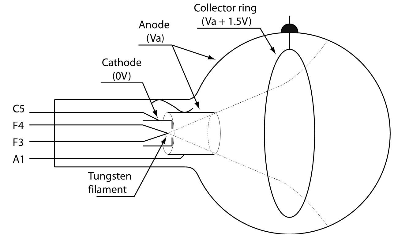 |
| Figure 1: Geometry of the critical potential tube |
The anode is held at a potential, $V_a$, which is more positive than the cathode. Thus, electrons generated at the cathode are accelerated to a kinetic energy of $K = eV_a$ by the time they reach the anode can. In the absence of any collector ring potential and with no helium atoms present, the electrons would continue, undeflected, to the inside of the glass tube. However, since the collector ring is held at a potential 1.5 V more positive than its surroundings, the electrons are attracted toward the collector ring as they pass it. The aperture of the anode cylinder is such that these electrons would miss the collector ring.
In our experiment, we will increase $V_a$ linearly with time. Thus, the electron energy will also increase with time. Collisions between electrons and helium atoms will occur, but as long as the electron energy is less than an atomic excitation energy, these collisions will not result in significant energy absorption by the atom. Electrons scattered in this manner (elastically) are relatively unlikely to reach the collector ring, since they will have energies nearly equal $V_a$.
An electron whose energy is reduced to less than 1.5 eV by exciting a helium atom will be attracted to the collector ring, and will contribute to a measured negative current. On the other hand, electrons not exciting atoms will miss the ring and continue to the anode on the inner surface of the tube.
A note on mean free path:
The helium pressure and the geometry of the tube play a linked role in the design of the apparatus. The mean free path is defined as the average distance an electron must travel between collisions with helium atoms. Thus, the mean free path is determined by the helium pressure.
In this tube, the helium pressure has been set so that there is a small probability of collision in the region between the cathode and the cylindrical anode (where the electrons are being accelerated), but a large probability for a collision thereafter (where the electrons are traveling at constant speed). Thus, when the collisions take place, the electron energy is well known.
A note on the work function and contact potential difference:
As electrons leave or enter a metal surface, they are subject to electric field gradients due to the charges present in the metals. The potential barrier caused by these field gradients is called the work function of the metal. Work functions differ for different metals. In our tube, electrons leave the cathode and enter the anode, and will experience field gradients at both interfaces. The net effect of these gradients is called contact potential difference (CPD). The CPD will effectively increase or reduce the accelerating voltage, depending upon their signs and magnitudes.
Helium transition energies
Table 1 gives the wavelengths emitted by transitions from the lower excited states to the ground state of helium. It is important to note that these wavelengths were measured spectroscopically. Only later were they converted to energies using the Planck relation, $E = hc/\lambda$.
Recall that, at the time of the Franck-Hertz experiment in 1914, the Planck relation was only an assumption, used to “fudge” the black-body theory. An independent method to measure energies was needed to verify the Planck relation. You are here to measure those energies!
For the hypothetical atom in the prelab, we ignored the spin of the electron. Here, it will be important to keep track of the spin because the orientation of one electron (relative to the other) adds an additional small separation in the energy levels.
- An electron has an intrinsic spin of s = 1/2.
- Neutral helium has two electrons. Therefore the total spin can be either $S = 0$ (if the spins point in opposite directions) or $S = 1$ (if the spins point in the same direction).
- An atom where $S = 0$ (electrons in opposite directions) is called parahelium.
- An atom where $S = 1$ (electrons in the same direction) is called orthohelium.
- Because of the Pauli exclusion principle, when both electrons are in the ground state they must have oppositely directed spins; therefore, the ground state is parahelium.
In Table 1 below, we are using the expanded spectroscopic notation $n^{2S+1}L$, where $n$ is the principle quantum number, $S$ is the total spin, and $L$ is the angular momentum quantum number (such that S is L = 0, P is L = 1, and D is L = 2). In this notation, an excited state $n^3L$ is an orthohelium state and $n^1L$ is a parahelium state.
| Excited state ($n^{2S+1}L$) | Wavelength (measured by spectroscopy), $\lambda$ (nm) | Energy (calculated), $E = hc/\lambda$ (ev) |
|---|---|---|
| $2^3S$ | 62.559 | 19.82 |
| $2^1S$ | 60.143 | 20.62 |
| $2^3P$ | 59.144 | 20.97 |
| $2^1P$ | 58.435 | 21.22 |
| $3^3S$ | 54.576 | 22.72 |
| $3^1S$ | 54.095 | 22.92 |
| $3^3P$ | 53.891 | 23.01 |
| $3^3D$ | 53.740 | 23.07 |
| $3^1D$ | 53.740 | 23.07 |
| $3^1P$ | 53.706 | 23.09 |
| $4^3S$ | 52.551 | 23.59 |
| $4^1S$ | 52.375 | 23.67 |
| Ionization ($\infty$) | – | 24.587 |
| Table 1: Energy levels and resonance energies of helium. | ||
These wavelength measurements were taken originally from the book A.R. Striganov, N. S. Sventitskii, Tables of Spectral Lines of Neutral and Ionized Atoms, 1968 (a.r._striganov_n._s._sventitskii_-_tables_of_spectral_lines_of_neutral_and_ionized_atoms_-_1968a.pdf), and are quoted (along with energy calculations) in N. Taylor et. al., “Energy levels in helium and neon atoms by an electron-impact method”, Am J Phys 49(3), March 1981 (franck-hertz-ajp.pdf).
The ionization energy is taken from the NIST Atomic Spectra Database and truncated to three decimals. That measurement is from a 2011 paper(Extreme Ultraviolet Frequency Comb Metrology) and is precise down to better than than 1 part in 1,000,000,000.
Prelab exercises
Consider a hypothetical atom that has the following electron energy diagram.
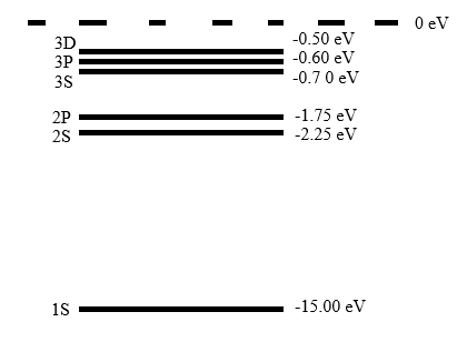 |
Recall that when designating an energy level as nL, n represents the principal quantum number and L represents the orbital angular momentum quantum number. For historical reasons, L is not written as a number but as a letter following the convention $S$ for $L = 0$, $P$ for $L = 1$, $D$ for $L = 2$, and $F$ for $L = 3$. These electron clouds have different shapes (or distributions) which mean that different L orbitals have slightly different energies, even within the same principal energy level.
In order for an electron in the ground state (1S) to be excited to one of the higher energy states, it must receive an amount of energy $\Delta E$ equal to the difference between its initial (ground) and final (excited) state.
- (1) Given the above energy diagram, what are all the energy differences that correspond to transitions from the ground state to the excited states shown? (Ignore any “selection” rules you might have learned. For this exercise, suppose that all we need to do is satisfy the energy difference.)
- (2) How much energy would be needed to ionize the atom (i.e. to eject the electron from the atom completely)?
Now suppose that our critical potential tube (as illustrated in Fig. 1) is filled with this hypothetical gas (instead of helium). You collect the following data.
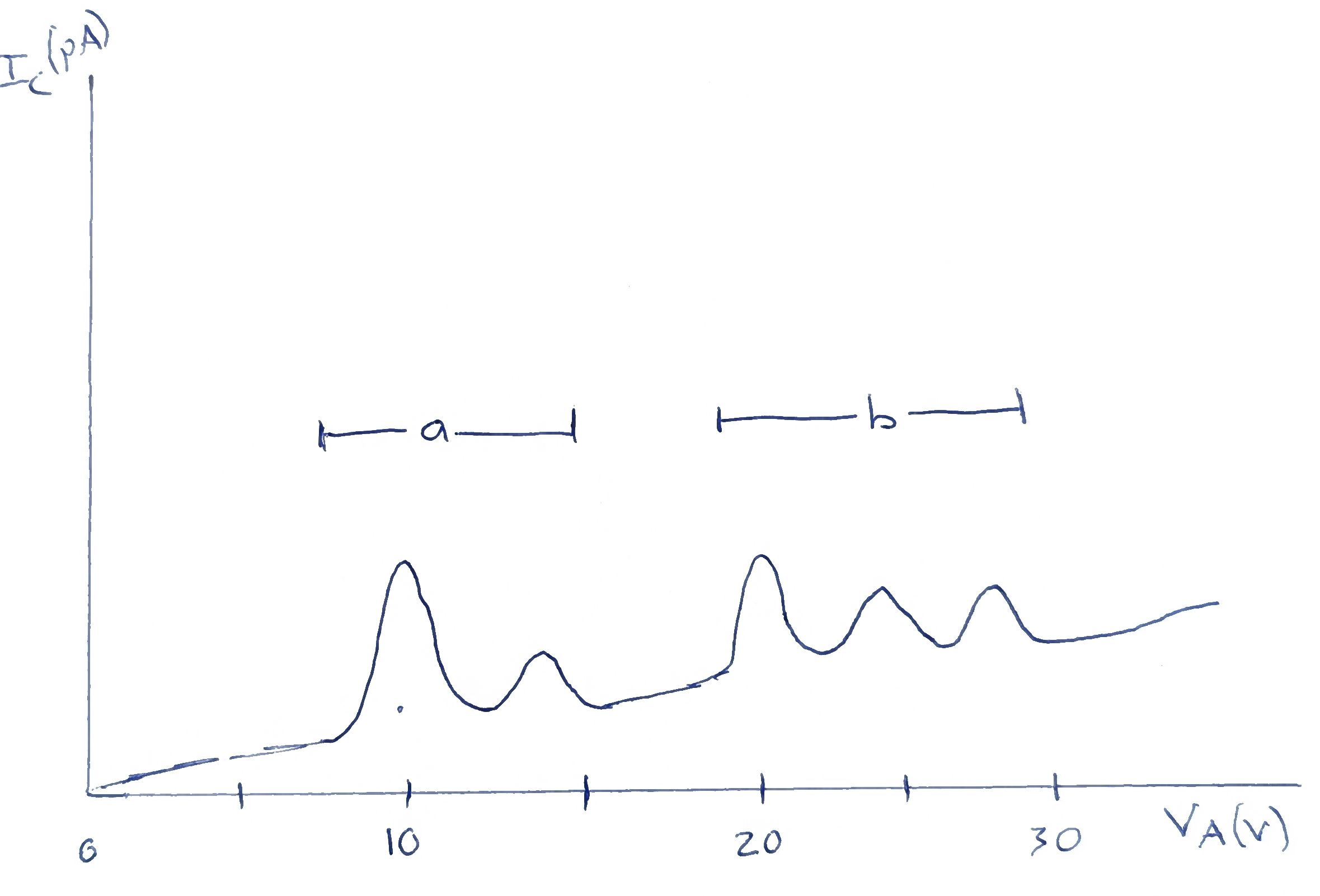 |
- (3) What is happening in region (a) of the plot?
- (4) What is happening in region (b) of the plot?
Day 1: Familiarizing yourself with the apparatus
Lab notebook
You are expected to keep a record of your work in a permanent lab notebook. There is no exact formula for what should go into a lab notebook. A good rule of thumb is to record everything which you would need to refer back to if you wanted to exactly reproduce your experiment at a later time, or that you might need to know when writing a paper on your results or explaining to a colleague what you did and how you did it.
For this experiment you should record voltages and equipment settings while you test that the apparatus is functioning correctly. Once you are concentrating on collecting data, you will need to make sketches of your scope traces, record the accelerating voltage ranges and scope settings, and keep track of scope readings and/or saved files. After you leave the lab and sit down to do your analysis, you likely will not remember all of these details, so it it critical to record them.
We recommend (highly!) that while you are in the lab collecting data you should be doing calculations and making quick plots of the data in order to evaluate how things are going and ascertain any corrections you may need to make. These calculations and plots should all go into your lab notebook.
Electrical connections
The Hertz tube console is used to control the accelerating potential, $V_a$, and read the current from the collector ring. The accelerating voltage is supplied as a sawtooth ramp of frequency 20 Hz.
- The minimum and maximum voltages of the ramp can be set from 0 V to +60 V, using the MIN and MAX controls on the right hand side of the console.
- Output FAST 1 provides an voltage proportional to the accelerating voltage, with a proportionality constant unique to each console: $V_1 =aV_a+b$, where $a$ and $b$ are constants.
- Output FAST 2 provides an voltage proportional to the collector ring current such that 1 V corresponds to 1 pA, $V_2 = I_c/(1~\textrm{pA})$.
- Output 3 provides a voltage proportional to the maximum ramp voltage: $V_3 = V_{a, max}/1000$.
- Output 4 provides a voltage proportional to the minimum ramp voltage: $V_4 = V_{a, min}/1000$.
Note that a few control consoles have a design difference where outputs 3 and 4 have a proportionality constant of 1/2000 instead of 1/1000 such that $V_3 = V_{a, max}/2000$ and $V_4 = V_{a, min}/2000$. These devices are clearly marked with this difference.
A separate DC power supply provides current to the filament and a 1.5 V battery supplies a small potential to attract electrons to the collecting ring. A digital oscilloscope is used to view and measure the current in the collector ring and the accelerating voltage, $V_a$.
A full wiring diagram is shown in Fig. 2. However, rather than connect everything at once, it will be more instructive to work through the logic of the connections step-by-step.
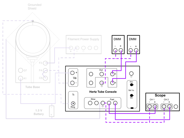 | 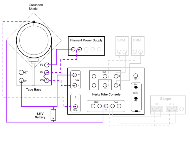 |
| Figure 2a: Connections to the multimeters and oscilloscope (click on image to enlarge) | Figure 2b: Connections to the critical potential tube (click on image to enlarge) |
Connecting multimeters and the oscilloscope
Multimeters
To begin, connect the two digital voltmeters that monitor the $V_{a,min}$ and $V_{a,max}$ values produced by the console.
- Plug the Hertz tube console into the wall outlet. (A light in the lower right corner will illuminate when the console is powered on).
- Connect one voltmeter to monitor the voltage at Output 3. To do so…
- …Connect the “V” side of the voltmeter to Output 3.
- …Connect the COM“ side of the voltmeter to any one of the ground (⏚) jacks on the console.
- …Turn the meter on to the DC voltage scale.
- Repeat with Output 4.
If everything is connected correctly, you should be reading voltage values from the two outputs in the range from 0 to 60 mV. Adjust the MAX and MIN control knobs and observe how the voltages change.
Oscilloscope
Next, connect the FAST Outputs 1 and 2 to oscilloscope Channels 1 and 2 in order to monitor the $V_a$ ramp voltage and the ring collector voltage, respectively. (We will not use the SLOW outputs on the console.)
- Turn on the oscilloscope.
- Using a BNC to double banana adapter, connect the red side of Channel 1 to FAST Output 1 and connect the black side of Channel 1 to any ground (⏚) jack on the console.
- If you get this backwards you may not see any signal on the scope!
- Repeat with Channel 2.
At the moment, Channel 2 should be a flat signal at 0 V (as the collector ring is not yet attached to the console). However, Channel 1 should display a sawtooth voltage signal with a frequency of 20 Hz (or period of 1/20 Hz = 50 ms).
- Trigger the scope on Channel 1 to achieve a stable trace.
- Suggestion: Trigger on the falling slope of Channel 1 in order to catch the sawtooth cleanly at the start of each cycle. If you attempt to trigger on the rising slope, you may find that noise in the signal causes the trace to jiggle around from trigger event to trigger event. If you find that your trace is acting this way, use the “high frequency” reject setting (found in Trigger Menu: More: Coupling: HF Reject).
- Adjust the Channel 1 voltage and time base to fill the screen with a single $V_a$ ramp.
- Adjust the $V_{a, min}$ and $V_{a,max}$ knobs on the console while observing the effect on the scope.
Checkpoint: Calibration
You may notice that the voltages displayed on the oscilloscope at the maximum and minimum of the ramp do not match the voltages you read on your meters ($V_3$ and $V_4$), nor do they match the actual $V_a$ maximum and minimum values. As a result, you will need to calibrate; when you collect data, you will record scope voltage measurements $V_{scope}$, but you will need to determine a conversion formula between those values and the actual $V_a$.
- Figure out how you can use the MIN and MAX adjustments on the console – along with meter readings $V_3$ and $V_4$ – to determine the relationship between $V_{scope}$ and $V_a$.
- Estimate the uncertainty in your voltage calibration.
You may want to discuss your results with a TA before moving on.
Connecting the critical potential tube
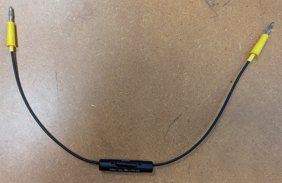 |
| Figure 3: The wire with the in-line fuse (to be used as one connection from power supply to filament) |
Now connect the tube to the console.
With the filament power supply OFF, connect the supply to the tube base.
- Connect the positive side of the power supply (red) to jack F3 on the back of the tube base.
- Use the cable with the in-line fuse (shown in Fig. 3) to make this connection. This will protect the filament if it attempts to draw too much current.
- Connect the negative side of the power supply (black) to jack F4 on the back of the tube base.
Do not turn the power supply on yet. It is possible to damage or destroy the filament by running too much current.
Do not connect any wires to the ground (green) jack on the power supply. The ground of the power supply (which is connected to the third prong in the wall outlet) is different from the ground potential of the console.
Next, connect the anode and cathode to the $V_a$ ramp…
- Connect $V_A$ Output 1+ (in the box in the upper left corner of the console) to jack A1 on the back of the tube base. (This is the anode voltage.)
- Connect $V_A$ Output 1- to jack C5 on the back of the tube base. (This is the cathode voltage.)
- Connect the short green jumper wire between jack C5 and jack F4. (This ties the low voltage side of the filament circuit to the cathode voltage.)
- NOTE: This connection is made internally on some of the tube bases already. This jumper guarantees the connection in case your tube base is one of the ones where the internal connection is missing.
In order to maintain the ring collector at +1.5 V relative to the anode, connect a AA battery between the anode and ground.
- Connect the negative side of the battery holder to the anode (either jack A1 on the tube base or $V_A$ Output 1+ on the console).
- Connect the positive side of the battery holder to any ground jack on the console.
Finally, connect the ring collector to the console.
- Connect the BNC cable from the top of the tube to INPUT 2 on the console (in the box in the lower left corner of the console).
With the ring current now connected to the console, you should observe a signal on Channel 2 of the oscilloscope. (Zoom in if the signal still appears flat.) The signal will likely be noisy (and may also have a periodic component with a frequency of 60 Hz) because the ring is collecting any stray electrons from the room which pass through the tube near the ring. In order to suppress this background noise, we can use a grounded shield which will intercept these electrons and direct them to ground (instead letting them pass through the tube to be picked up by the ring).
- Slide the carboard and metal shield around the tube, making sure that the tab slides into the grove along the tube base and the shield is pushed all the way back so that it fully covers the tube.
- Connect the wire from the shield to any ground jack on the console.
With the shield in place, the signal on the scope should now be much less noisy (though likely still not quite flat).
Observing helium excitation
Before turning on the filament, we need to make one more adjustment to the oscilloscope. Under the Channel 2 menu, select Invert: On. This will multiply the voltage measured on Channel 2 by -1 (thus inverting the signal). By the manufacturer's conventions, the collector ring current circuit is outputs a negative voltage (proportional to current), though it will be more intuitive to look at and interpret the signal as a positive voltage (current).
It is now time to turn on the tube and begin to look for critical potential dips.
- With the filament power supply still off, turn the current knob fully up (all the way clockwise) and the voltage knob fully down (all the way counter-clockwise).
- This ensures that the power supply will begin in constant voltage mode. (See below for more info on constant voltage versus constant current mode.)
- Turn the power supply on.
- Slowly increase the voltage (by turning the voltage knob only).
- You should observe that as the voltage reaches about 2-3 V (or as the current reaches about 0.75-1.0 A), the Channel 2 signal on the scope should begin to change (as the ring collector begins to pick up electrons produced inside the tube instead of just noise).
- At first the signal may look just have a general negative trend, but you should be able to discern two or three groups of dips superimposed on this general background. These are the critical potential dips!
- You may continue increasing the voltage to enhance the signal. Keep an eye on the current! Do not exceed 1.2 A!
- The signal may fluctuate slightly in intensity as the filament warms up. It should stabilize after a few minutes.
If the observed signal is already smooth, it may be possible to make out all the details already. However, if the signal is noisy, you may want to implement averaging. (To turn averaging on, select Acquire: Average: N where N is the number of trigger events the scope will average over. You may need to select N = 16 or 64 if your signal is especially noisy.)
Constant voltage (CV) and constant current (CC) modes
A light on the front of the power supply will indicate whether the power supply is in constant voltage (CV) or constant current (CC) mode.
- When the power supply is in CV mode, it will attempt to maintain the voltage set by the voltage control knob by adjusting the current provided (up to the maximum current allowed by the current control knob).
- When the power supply is in CC mode, it will attempt to maintain the current set by the current control knob by adjusting the voltage difference (up to the maximum voltage difference allowed by the voltage control knob).
If you have no need to limit a voltage or current, then you can turn one of the knobs up to maximum and control the power supply by the other knob. (Typically this means CV mode… so turning current to max and using the voltage knob to adjust.)
If, however, you wish to limit a voltage or current (for example to prevent a fuse from blowing or to protect a sensitive circuit), then you can turn the corresponding knob down to a lower lower level.
In this experiment – where we wish to make sure we never exceed about 1.2 A of current – we can set this limit by slowly turning up the voltage knob until we reach a reading of about 1.2 A. Then, we can slowly turn down the current knob until the light on the front of the supply changes from CV to CC. At that point, the supply is now limited to about 1.2 A and you should not be able to exceed that amount no matter what the voltage setting.
Interpreting the ring collector signal
You should notice that there are two or three groups of small peaks superimposed on the positively increasing collector ring signal. These peaks represent increases in the collector ring current that occur when the accelerated electrons have just enough kinetic energy to excite an electron in a helium atom from the ground state up to one of the excited electronic levels. After colliding with the atom and giving up this energy, the electron (now with $K=0$) is attracted to the ring.
Why is there a slowly increasing background trend?
First, the flux of electrons emitted by the filament wire increases as the accelerating potential increases. The electron current density, $J$, (in units of current/area) is given by a formula known as Child's Law,
| $J = k V_A^{3/2}$, |
where $k$ is a proportionality constant that depends on the mass of the electron, the charge of the electron, and the separation distance between the anode and cathode.
Child's law is a consequence of the space charge limiting effect. The first electrons to be emitted from the filament when it is heated form a “cloud” around around the wire known as space charge. The negative electric potential created by this cloud makes it harder for future electrons to be ejected. However, as the potential between anode and cathode is increased, this repulsive effect is reduced, leading to the increase in the flux of electrons emitted.
Second, even though the trajectories of the accelerated electrons form a cone that does not intersect with the collection ring (see Fig. 1), it is always possible that an electron undergoes an elastic scatter off a helium atom and changes direction. As the flux of electrons increases, the number of electrons that are randomly scattered into the collection ring increases proportionally.
Therefore, since the electron flux increases as $V_A^{3/2}$, the background upon which the peaks appear also should increase as $V_A^{3/2}$.
What's going on with the first set of peaks?
As was the case in the prelab question, the first set of peaks corresponds to the minimum energies required to excite an electron from the ground state of helium up to one of the possible excited states. As there are many possible excited states, there are many possible excitation energy peaks… though just as in the prelab, some of these energies may be so closely spaced that we can't distinguish them as separate and they instead merge together into one peak.
We will spend more time on Day 2 investigating these individual dips, but for now let's focus just on the first dip (as the mark of the beginning of these possible excitations).
What's going on with the second set of peaks?
For the second set of peaks, the interpretation is a bit more complicated. Here, electrons have enough energy to excite two different atoms.
- Some of the electron energy excites atom 1 from ground to some excited state.
- The rest of the energy goes to atom 2 to excite it from ground to an excited state.
- The total energy the electron started with is the sum of those two excitation energies.
- Since there are multiple possible excitations for each atom ($1^1S \rightarrow 2^1S$, $1^1S \rightarrow 2^1P$, etc.), there will be an energy peak in the second set corresponding to each pair of transitions.
- The resulting set of peaks will therefore look similar to the first set of peaks, but you should notice that there are more peaks overall (and that the intensities of those peaks differ).
Given the complexity of this spectrum, we won't try to identify each peak. Again, for now let's focus just on the first dip (as the mark of the beginning of these possible two-atom excitations).
Measuring peak positions
Adjust $V_{a,min}$ and $V_{a,max}$ so as to zoom in on the group of peaks at the lowest $V_a$ on the scope. (You may have to adjust the scope trigger level to keep the peaks centered on the display.) If the peaks are weak, adjust the filament voltage – without exceeding 1.2 A – to maximize the number of peaks visible in this group. Adjust the voltage scale on Channel 2 so that the peaks fill as much of the display as possible. If needed, average over trigger events to capture a spectrum of peaks and the accelerating voltage ramp.
- Use the voltage cursor to measure the ramp voltage at the position of the first peak. Use your calibration to covert this voltage to a $V_a$ value.
- Repeat this process, zooming in on the second set of peaks and measuring the position of the first peak in that group.
Checkpoint: Interpretation of the signal // Saving your signals
As you will have to interpret your signal for the analysis, you should stop and make sure you can answer the following questions.
- Why are there multiple groups of peaks?
- What is significant about the first peaks in each group?
- If our accelerating voltage went high enough, would we expect a third group of peaks? A fourth?
Speak with a TA if you aren't sure. Save screenshots of your signals (by using the scope transfer or USB thumb drive procedures introduced in the introductory scope skills lab last week). You may also want to save the raw scope data csv files (t vs. V for channels 1 and 2). Make sure to capture at least the three following scenarios:
- A wide sweep that shows both the first and second sets of peaks (along with the corresponding voltage ramp).
- A zoomed-in sweep that shows only the first set of peaks (along with the corresponding voltage ramp).
- A zoomed-in sweep that shows only the second set of peaks (along with the corresponding voltage ramp).
In your analysis, you will need to visually identify features in the signal. Make sure you have what files you need before leaving the lab.
Contact potential difference
Recall from the note in the introductory material that “as electrons leave or enter a metal surface, they are subject to electric field gradients due to the charges present in the metals. The potential barrier caused by these field gradients is called the work function of the metal. Work functions differ for different metals. In our tube, electrons leave the cathode and enter the anode, and will experience field gradients at both interfaces. The net effect of these gradients is called contact potential difference (CPD). The CPD will effectively increase or reduce the accelerating voltage, depending upon their signs and magnitudes.”
This means that the voltage corresponding to the first peak in the first set of peaks does not actually correspond to the true accelerating voltage for that electron; it instead is the true potential plus the CPD (which may be positive or negative). If we designate the measured voltage of the first peak in the first set as $V_0$, the contact potential difference as $V_{CPD}$, and the true voltage of the first transition as $V_{0,true}$, we have the relation
| $V_0 = V_{0,true} + V_{CPD}$. | (1) |
Thinking now about the second set of peaks, the measured voltage of the first peak in that group is (using the same subscript conventions)
| $V_0^{\prime} = 2V_{0,true} + V_{CPD}$. | (2) |
Putting Eqs. (1) and (2) together, we can solve for the true voltage required for the transition as
| $V_{0,true} = V_0^{\prime} - V_0$, | (3) |
and then solve for the CPD as
| $V_{CPD} = 2V_0 - V_0^{\prime}$. | (4) |
Once the CPD is known, you can now correct the systematic offset in the measurement of the peak positions in the first group.
Checkpoint: Calculating CPD
Collect data from both the first and second sets of peaks as needed to compute the contact potential difference (as described above).
- What do you calculate as the CPD for you system?
- What do you calculate as the minimum excitation energy, $E_{0,true} = eV_{0,true}$?
- Is this value in agreement with the literature value of $E_{0,true} = 19.82~\textrm{eV}$? (We will dive deeper into the electron structure of helium and the corresponding excitation energies in Day 2.)
Check with a TA if you need help with these tasks.
Day 1 Analysis
Day 1 Analysis
You now have some preliminary data to explore. Just as in a professional research lab, your work is not done yet. Analyze what you have (keeping in mind that we are not looking for the right answer… or even the complete answer yet.) The results of your analysis will likely generate new questions, and you will be able to use Day 2 to make improvements, repeat measurements, extend your experiment, or… do all of the above.
Complete the following set of analysis exercises and submit by 11:59 pm the day before you are due back in lab. Do not respond in bullet points or isolated text; respond in full sentences and paragraphs, and format your responses appropriately. Because this is your first analysis for the class, we have tried to be very explicit in what we are looking for and have provided prompting questions.
For each item below, include whatever data, plots, calculations, etc. you used in your determination. (If something is used in more than one item, you do not need to present it each time; you may reference plots, data, equations, etc. that you provided earlier in the analysis if that is appropriate.)
- Present your calibration between measured scope voltage and accelerating voltage.
- Explain why you need to calibrate and describe your calibration method. (See below for additional guidance.)
- Include an explicit final conversion equation from measured quantity to desired quantity.
- Provide a sketch, photo, or replotted scope trace of the current signal for the following three cases: all the peaks, a zoomed-in version that highlight just the first set of peaks, and a zoomed-in version that highlights the second set of peaks.
- Identify the first peak in each set, and provide your measured (and calibrated) value for those peak positions (along with uncertainties). Annotate or note the corresponding peaks on your figures.
- In your own words, what do these peaks represent? (Or put in other ways, what is physically happening at a point where a peak occurs, or why do we get a peak in the collector current at all?) Be as clear and explicit as you can.
- Explain how you measured/estimated these feature positions.
- Explain how you determined uncertainties (and differentiate between statistical uncertainties and systematic uncertainties, if you had any.)
- Determine the contact potential difference, $V_{CPD}$ and the minimum excitation energy, $E_{0,true} = eV_{0,true}$.
- Compare your value of $E_{0,true}$ to the literature value. Are you in agreement?
- Now that you have completed your initial analysis, what would you like to do differently when you return to lab for the second day? Below are some suggestions to consider. You don't need to answer all the questions; address whichever you think are appropriate.
- Is there anything in how you collected data that you would like to check or change?
- Are there more or different data that you would like to collect?
- Are there any side/auxiliary experiments that you'd like to carry out, or any hypotheses that you'd like to explore?
- Is there anything in how you analyzed the data that you would like to retry or change?
- Are there any questions you have or is there anything you want to know that would require you to seek outside resources or research? This could mean any of the following:
- data – e.g. literature values of certain quantities (other than the excitation energies you're trying to measure)
- technical specifications – e.g. information about your apparatus (helium tube or console electronics) or your measurement tools (scope or multimeter)
- physics theory or models – e.g. quantum theory about atomic energy levels or about inelastic electron scattering
- etc.
Guidelines for discussing your calibration
When we ask you to do something for your analysis that you have not done before, we will try to provide you with more explicit guidance so that you understand what we are looking for (and so we can model how a professional physicist thinks through the discussion of different types of results).
For this analysis, the item most likely to be new to you is the requested “discussion of your calibration”. In discussing a particular experimental procedure like calibration, the goal is to make clear to the reader both why you performed a calibration and how you performed it.
Some things to consider include the following:
- Why was it necessary to perform this calibration?
- What was the quantity you needed, what quantity(s) did you actually measure, and how were they related to one another?
- How did you determine the value of each of your measured quantities? (Did you read a ruler and interpolate between tic marks by eye? Did you use an automated scope feature to perform your measurement? Something else?)
- What limited how well you could perform these measurements, and what did you do to assess how well you were able to measure them?
- What did you do with the data you collected? Did you use it to determine a conversion equation, or did you use it to determine a setting on some piece of apparatus?
The above is not a bullet point checklist to be filled out; we are looking for you to articulate clearly and concisely the what, why and how of your calibration. The better you understand what you were doing, why you were doing it, and how you did it… the easier this task will be.
More generally, whenever describing procedure or attempting to justify or explain a technique, keep the following in mind:
- Avoid word salad: Don't use unnecessary jargon just because it “sounds” scientific. Make sure you know what terms mean and that you are using them correctly.
- When using a new term, define it. Sometimes, when forced to articulate a piece of jargon, you realize that you do not understand it yourself or that you are not using it correctly (and you can use this moment to correct your own understanding).
- Whenever possible, it is preferable to explain something fully (so that the reader understands) than to use a shortcut word or phrase (that the reader may be confused about).
- If you find your explanation getting long or complex, break it up into smaller chunks (e.g. shorter sentences or paragraphs).
- Consider flow: Though we are not looking for a full report or article, each piece of your analysis needs to have a logical flow and be easy to follow.
- Think about the order it makes sense to talk about things in (which is often different from the order you did things in.)
- Think about what is necessary to make your point, and omit anything that doesn't contribute to the argument. (Just because you did something in lab does not mean you need to talk about it, and including extraneous information can make it harder for the reader to follow your story.)
- If a grader has to read through a passage multiple times to make sense of what you are writing, you will lose credit (even if your description is technically complete and correct). The purpose of these analysis is to communicate, not to prove that you got the “right answer”.
Day 2: Additional measurements
On Day 2, you will repeat your data collection, implementing any changes you want to make based on the results of your previous analysis. In addition, you will dig down into the details of signal in order to measure individual peak positions and try to identify the different possible excitation energies.
You may wish to remind yourself of the expected helium electron transitions shown in Table 1 (in the “Helium transition energies” dropdown in the “Before you come to lab…” section) before beginning.
Things to keep in mind
You will collect a fresh set of data. Are there any changes you want to make from how you collected data on Day 1? For example…
- Were there any systematic effects you believe may have affected your measurements that you can explore or quantify today?
- Is there any way to make more precise measurements (i.e. to reduce the statistical uncertainties)?
- Are there data you need to save or record that you did not save or record on Day 1?
Even if you are completely happy with your data and data collection strategy from Day 1, you should collect a fresh set of data. If nothing else, it will give you a feeling for how reproducible the results are or how results may fluctuate from day to day (or from apparatus to apparatus).
Determining individual helium excitation energies
Rewire your apparatus and adjust your settings to recover the helium excitation signal you saw on Day 1. Once you have a clear signal, zoom in on the first set of dips and optimize your signal.
Resolution
You likely noticed on Day 1 (and if not, you can look at your trace now) that the peaks are not sharp delta functions, but instead have some “width” to them. This limits how close together two features can be before the cease to be resolvable (i.e. distinguishable as two separate features instead of one single feature).
There are several valid definitions of resolution, but for this experiment we will define is as the full width at half-maximum (FWHM) of that peak. It is useful to measure (or otherwise predict) the resolution of your measurement apparatus so that you know the limitations of what data you can collect.
Checkpoint: Measuring resolution
To determine resolution…
- Zoom in on the first peak of the first group of peaks.
- Measure the full width half maximum of this peak. (No uncertainty on this value is required.)
- Convert the width (in units of voltage) to an energy (in units of eV).
NOTE: Since the FWHM value is small, the voltage ramp difference will also be small. You will likely need to to zoom in quite a lot on Channel 2 (the $V_a$ voltage ramp) so that it covers more of the height of the scope screen. If you attempt to make a measurement without zooming in, the voltage difference may appear to be zero).
Now consider the following:
- How does the resolution compare to the difference between excitation energies in helium (Table 1)? Are there any differences that are too close to be resolved?
- Are there any features in the data you collected that appear to be made up of multiple overlapping peaks?
- Can you think of any methods that could be used to determine two (or more) overlapping energies even if they are not visually resolvable?
Measuring peaks
Next we wish to identify as many helium excitation energies as we can.
- Using whatever methods you would like, measure as many distinct peak positions as you can within the first set of peaks. (Estimate uncertainty on each measurement.)
- You should be able to make out at least 4 distinct peaks. The fourth one is sometimes faint, so tune your signal (and use averaging) if needed to tease it out.
- In addition, measure the position of the first peak in the second set of peaks so that you can find the contact potential difference (CPD).
- Remember that because the CPD is a constant offset to all measured voltages, you will need to correct the measurements you make for each position within the first set of dips by subtracting off the CPD voltage.
In addition, we can make a (somewhat crude) estimate of the helium ionization energy. (This is the energy required to eject an electron completely from the atom instead of exciting it from ground to some intermediate state. You may find it helpful to think of the ionization energy as the energy required to excite the electron from its ground state to the $n = \infty$ state.)
Look at the end of the first set of peaks. Where does the series of peaks end? Does there appear to be a slight “kink” in the background at this point (where the background appears to increase slope)? This marks the onset of ionization (where we begin to collect some of the low-energy electrons ejected by helium in addition to electrons randomly scattered into the collection ring).
Checkpoint: Measuring helium excitations
Collect data (and save scope traces or screenshots) as needed to complete the following:
- Determine the CPD (as done on Day 1).
- Determine the excitation energies of as many peaks as you can (within the first set of peaks) and compare them to the known excitation energies given in Table 1.
- Determine the ionization energy of helium, and compare it to the value shown in Table 1.
Check with a TA if you need help with these tasks.
Directly measuring the ionization potential
While we are able to get a crude estimate of the ionization energy from the signal we have been looking at, there is another trick we can use. If the 1.5 V potential between the anode and the collecting ring is reversed – so that the collecting ring is now 1.5 V negative relative to the anode – the apparatus will collect positively charged ions instead of low energy electrons. When $V_a$ reaches the ionization potential (i.e., accelerated electrons have enough energy to eject an electron completely from a helium atom), the resulting positively-charged helium ions will be collected by the negatively biased collector ring.
To measure the ionization potential, reverse the 1.5 V battery in its holder so that the positive terminal is now connected to the tube anode. Observe the signal on the scope and adjust $V_{a,min}$, $V_{a,max}$, and the filament voltage until you obtain a signal from the collector ring with the features shown in Fig. 4.
NOTE: Because the particles collected by the ring have opposite sign from earlier (positive ions instead of negative electrons), the current produced by the ring also has an opposite sign. You may wish to undo the inversion of your Channel 2 signal (i.e., select Invert:Off in the Channel 2 menu) so that your current signal is again a positive-definite value.
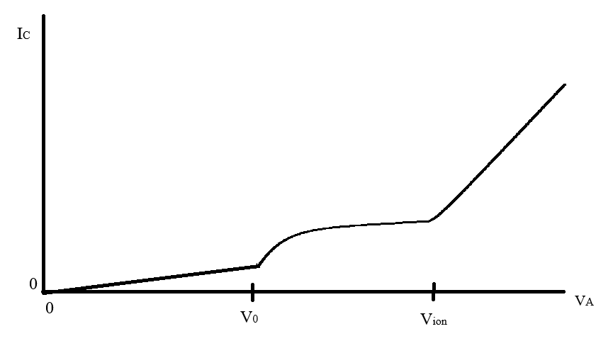 |
| Figure 4: Features of ionization curve |
At accelerating voltages below $V_0$ (the energy corresponding to the lowest electron excitation energy), your current signal will likely be flat or nearly flat. As $V_a$ increases from $V_0$ to $V_{ion}$, the signal will increase as some helium atoms are ionized in the following two collision process: the first collision puts the atom in a metastable excited state and then – before the atom can decay back to the ground state – a second collision knocks the electron out of the excited state, ionizing the atom. (This ionization of the metastable state is not what we are trying to measure.) The abrupt change in slope that occurs at $V_{ion}$ represents the onset of ionization from the ground state.
Checkpoint: Measuring the ionization potential
Collect data as needed to determine the ionization potential. You may need to adjust $V_{a,min}$ and $V_{a,max}$ in order to get close to the ionization point to observe the “kink” in the slope of the current.
- Save screenshots (or raw csv files) of your scope traces, and make sketches in your lab notebook.
- Measure the onset of ionization (and/or any other features you wish) from the scope and record them in your notebook.
Check with a TA if you need help with these tasks.
Day 2 Analysis
Day 2 Analysis
For your Day 2 analysis, complete the following set of analysis exercises and submit by 11:59 pm the day before you are due back in lab. Note that some of the tasks are identical to Day 1, but you should use your Day 2 data here (and any improved data collection or analysis methods you wish to apply).
For each item below, include whatever data, plots, calculations, etc. you used in your determination. (If something is used in more than one item, you do not need to present it each time; you may reference plots, data, equations, etc. that you provided earlier in the analysis if that is appropriate.)
- Present your calibration between measured scope voltage and accelerating voltage.
- Include an explicit final conversion equation from measured quantity to desired quantity.
- You do not need to repeat your explanation of the calibration method from Day 1; just present your results.
- Provide a sketch, photo, or replotted scope trace of the current signal for the following three cases: all the peaks, a zoomed-in version that highlight just the first set of peaks, and a zoomed-in version that highlights the second set of peaks.
- Identify (and provide measurements with uncertainties for) the following:
- The four peak positions in the first peak set.
- The first peak position in the second peak set.
- The position where ionization occurs.
- Annotate or note the above features on your figures.
- Explain how you measured/estimated the positions.
- Explain how you determined uncertainties (and differentiate between statistical uncertainties and systematic uncertainties, if you had any.)
- Determine (and explain your measurement/calculation of) the contact potential difference, $V_{CPD}$.
- Determine the resolution of the first peak in the first set of peaks. (No uncertainty on this value is required.)
- Explain your method for determining FWHM and include data, plots and calculations as needed.
- Compare your results to the calculated excitation and ionization energies of helium provided in Table 1.
- Were you able to observe and measure all the individual energies listed?
- If not, why do you think that is? (What role does resolution play?)
- Are your values in agreement with the values in the table?
- If not, is your disagreement random (i.e. some values are too high and some are too low) or systematic (i.e. all values trend too high or too low)?
- Using the plot obtained when you reverse the collector ring potential, determine the ionization energy for helium.
- Is your result from this measurement consistent with the ionization energy determined above? Is it consistent with the literature value?